Summary: “The physics of the Earth’s atmosphere” Papers 1-3

Introduction

We have written a series of three papers discussing the physics of the Earth’s atmosphere, and we have submitted these for peer review at the Open Peer Review Journal:

1. The physics of the Earth’s atmosphere I. Phase change associated with the tropopause – Michael Connolly & Ronan Connolly, 2014a
2. The physics of the Earth’s atmosphere II. Multimerization of atmospheric gases above the troposphere – Michael Connolly & Ronan Connolly, 2014b
3. The physics of the Earth’s atmosphere III. Pervective power – Michael Connolly & Ronan Connolly, 2014c

In these papers, we show that carbon dioxide does not influence the atmospheric temperatures. This directly contradicts the greenhouse effect theory, which predicts that carbon dioxide should increase the temperature in the lower atmosphere (the “troposphere”), and decrease the temperature in the middle atmosphere (the “stratosphere”).

It also contradicts the man-made global warming theory, since the the basis for man-made global warming theory is that increasing the concentration of carbon dioxide in the atmosphere will cause global warming by increasing the greenhouse effect. If the greenhouse effect doesn’t exist, then man-made global warming theory doesn’t work.

Aside from this, the results in our papers also offer new insights into why the jet streams exist, why tropical cyclones form, weather prediction and a new theory for how ozone forms in the ozone layer, amongst many other things.

In this essay, we will try to summarise some of these findings and results. We will also try to summarise the greenhouse effect theory, and what is wrong with it.

However, unfortunately, atmospheric physics is quite a technical subject. So, before we can discuss our findings and their significance, there are some tricky concepts and terminology about the atmosphere, thermodynamics and energy transmission mechanisms that we will need to introduce.

As a result, this essay is a bit more technical than some of our other ones. We have tried to explain these concepts in a fairly clear, and straightforward manner, but if you haven’t studied physics before, it might take a couple of read-throughs to fully figure them out.

Anyway, in Section 2, we will describe the different regions of the atmosphere, and how temperatures vary throughout these regions. In Section 3, we will provide a basic overview of some of the key physics concepts you’ll need to understand our results. We will also summarise the greenhouse effect theory. Then, in Sections 4-6, we will outline the main results of each of the three papers. In Section 7, we will discuss what the scientific method tells us about the greenhouse effect. Finally, we will offer some concluding remarks in Section 8.

The atmospheric temperature profile

As you travel up in the atmosphere, the air temperature generally cools down, at a rate of roughly -6.5°C per kilometre (-3.5°F per 1,000 feet). This is why we get snow at the tops of mountains, even if it’s warm at sea level. The reason the air cools down with height is that the thermal energy (“heat”) of the air gets converted into “potential energy” to counteract the gravitational energy pulling the air back to ground. At first, it might seem hard to visualise this gravitational cooling, but it is actually quite a strong effect. After all, it takes a lot of energy to hold an object up in the air without letting it fall, doesn’t it?

This rate of change of temperature with height (or altitude) is called the “environmental lapse rate”.

Surprisingly, when you go up in the air high enough, you can find regions of the atmosphere where the temperature increases with altitude!

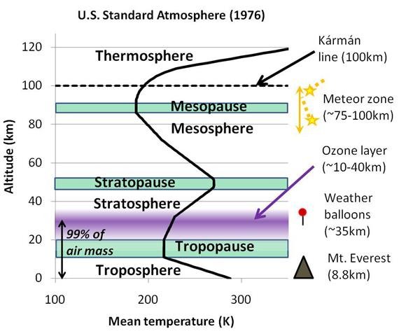
For this reason, atmospheric scientists and meteorologists give the different parts of the Earth’s atmosphere different names. The average temperature profile for the first 120 kilometres and the names given to these regions are shown in Figure 1.

By the way, in this essay we will mostly be using the Kelvin scale to describe temperatures. This is a temperature scale that is commonly used by scientists, but is not as common in everyday use. If you’re unfamiliar with it, 200 K is roughly -75°C or -100°F, while 300 K is roughly +25°C or +80°F.

At any rate, the scientific name for the part of the atmosphere closest to the ground is the “troposphere”. In the troposphere, temperatures decrease with height at the environmental lapse rate we mentioned above, i.e., -6.5°C per kilometre (-3.5°F per 1,000 feet).

Above the troposphere, there is a region where the temperature stops decreasing (or “pauses”) with height, and this region is called the “tropopause”. Transatlantic airplanes sometimes fly just below the tropopause.

As we travel up higher, we reach a region where temperatures increase with height. If everything else is equal, hot air is lighter than cold air. So, when this region was first noticed, scientists suggested that the hotter air would be unable to sink below the colder air and the air in this region wouldn’t be able to mix properly. They suggested that the air would become “stratified” into different layers, and this led to the name for this region, the “stratosphere”. This also led to the name for the troposphere, which comes from the Greek word, tropos, which means “to turn, mix”, i.e., the troposphere was considered a region where mixing of the air takes place.

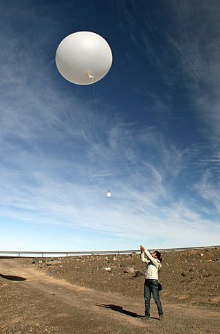
To get an idea of these altitudes, when Felix Baumgartner broke the world record for the highest skydive on October 14, 2012, he was jumping from 39 kilometres (24 miles). This is a few kilometres above where the current weather balloons reach, i.e., in the middle of the stratosphere:

At the moment, most weather balloons burst before reaching about 30-35 kilometres (18-22 miles). Much of our analysis is based on weather balloon data. So, for our analysis, we only consider the first three regions of the atmosphere, the troposphere, tropopause and stratosphere.

You can see from Figure 1 that there are also several other regions at higher altitudes. These other regions are beyond the scope of this essay, i.e., the “stratopause”, the “mesosphere” and the “mesopause”.

Still, you might be interested to know about the “Kármán line”. Although the atmosphere technically stretches out thousands of kilometres into space, the density of the atmosphere is so small in the upper parts of the atmosphere that most people choose an arbitrary value of 100 kilometres as the boundary between the atmosphere and space. This is called the Kármán line. If you ever have watched a meteor shower or seen a “shooting star”, then you probably were looking just below this line, at an altitude of about 75-100 kilometres, which is the “meteor zone”.

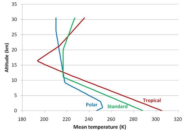
The temperature profile in Figure 1 is the average profile for a mid-latitude atmosphere. But, obviously, the climate is different in the tropics and at the poles. It also changes with the seasons. Just like ground temperatures are different at the equator than they are in the Arctic, the atmospheric temperature profiles also change with latitude. Typical temperature profiles for a tropical climate and a polar climate are compared to the “standard” mid-latitude climate in Figure 2, up to a height of 30 kilometres (19 miles).

One more term you may find important is the “boundary layer”. This is the first kilometre or two of the troposphere, starting at ground level. We all live in the boundary layer, so this is the part of the atmosphere we are most familiar with. Weather in the boundary layer is quite similar to the rest of the troposphere, but it’s generally windier (more “turbulent”) and the air tends to have more water content.

Crash course in thermodynamics & radiative physics: All you need to know

Understanding energy and energy equilibrium

All molecules contain energy, but the amount of energy the molecules have and the way in which it is stored can vary. In this essay, we will consider a few different types of energy. We already mentioned in the previous section the difference between two of these types, i.e., thermal energy and potential energy.

Broadly speaking, we can divide molecular energy into two categories:

1. Internal energy – the energy that molecules possess by themselves
2. External energy – the energy that molecules have relative to their surroundings. We refer to external energy as mechanical energy.

This distinction might seem a bit confusing, at first, but should become a bit clearer when we give some examples, in a moment.

These two categories can themselves be sub-divided into sub-categories.

We consider two types of internal energy:

1. Thermal energy – the internal energy which causes molecules to randomly move about. The temperature of a substance refers to the average thermal energy of the molecules in the substance. “Hot” substances have a lot of thermal energy, while “cold” substances don’t have much
2. Latent energy – the internal energy that molecules have due to their molecular structure, e.g., the energy stored in chemical bonds. It is called latent (meaning “hidden”), because when you increase or decrease the latent energy of a substance, its temperature doesn’t change.

   When latent energy was first discovered in the 18th century, it wasn’t known that molecules contained atoms and bonds. So, nobody knew what latent energy did, or why it existed, and the energy just seemed to be mysteriously “hidden” away somehow.

We also consider two types of mechanical energy:

1. Potential energy – the energy that a substance has as a result of where it is. For instance, as we mentioned in the previous section, if a substance is lifted up into the air, its potential energy increases because it is higher in the Earth’s gravitational field.
2. Kinetic energy – the energy that a substance has when it’s moving in a particular direction.

Energy can be converted between the different types.

For instance, if a boulder is resting at the top of a hill, it has a lot of potential energy, but very little kinetic energy. If the boulder starts to roll down the hill, its potential energy will start decreasing, but its kinetic energy will start increasing, as it picks up speed.

As another example, in Section 2, we mentioned how the air in the troposphere cools as you travel up through the atmosphere, and that this was because thermal energy was being converted into potential energy.

In the 18th and 19th centuries, some scientists began trying to understand in detail when and how these energy conversions could take place. In particular, there was a lot of interest in figuring out how to improve the efficiency of the steam engine, which had just been invented.

Steam engines were able to convert thermal energy into mechanical energy, e.g., causing a train to move. Similarly, James Joule had shown that mechanical energy could be converted into thermal energy.

The study of these energy interconversions became known as “thermodynamics”, because it was looking at how thermal energy and “dynamical” (or mechanical” energy were related.

One of the main realisations in thermodynamics is the law of conservation of energy. This is sometimes referred to as the “First Law of Thermodynamics”:

The total energy of an isolated system cannot change. Energy can change from one type to another, but the total amount of energy in the system remains constant.

The total energy of a substance will include the thermal energy of the substance, its latent energy, its potential energy, and its kinetic energy:

Total energy = thermal energy + latent energy + potential energy + kinetic energy

So, in our example of the boulder rolling down a hill, when the potential energy decreases as it gets closer to the bottom, its kinetic energy increases, and the total energy remains constant.

Similarly, when the air in the troposphere rises up in the atmosphere, its thermal energy decreases (i.e., it gets colder!), but its potential energy increases, and the total energy remains constant!

This is a very important concept to remember for this essay. Normally, when one substance is colder than another we might think that it is lower in energy. However, this is not necessarily the case – if the colder substance has more latent, potential or kinetic energy then its total energy might actually be the same as that of the hotter substance. The colder substance might even have more total energy.

Another key concept for this essay is that of “energy equilibrium”:

For a system in energy equilibrium, if one part of the system loses energy and starts to become unusually low in energy, energy flows from another part of the system to keep the average constant. Similarly, if one part of the system gains energy, this extra energy is rapidly redistributed throughout the system.

Is the atmosphere in energy equilibrium? That is a good question.

According to the greenhouse effect theory, the answer is no.

The greenhouse effect theory explicitly assumes that the atmosphere is only in local energy equilibrium.

If a system is only in local energy equilibrium then different parts of the system can have different amounts of energy.

As we will see later, the greenhouse effect theory fundamentally requires that the atmosphere is only in local energy equilibrium. This is because the theory predicts that greenhouse gases will cause some parts of the atmosphere to become more energetic than other parts. For instance, the greenhouse effect is supposed to increase temperatures in the troposphere, causing global warming.

However, this assumption that the atmosphere is only in local energy equilibrium was never experimentally proven.

In our papers, we experimentally show that the atmosphere is actually in complete energy equilibrium – at least over the distances from the bottom of the troposphere to the top of the stratosphere, which the greenhouse effect theory is concerned with.

What is infrared light?

Before we can talk about the greenhouse effect theory, we need to understand a little bit about the different types of light.

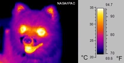
While you might not realise it, all warm objects are constantly cooling down by emitting light, including us. The reason why we don’t seem to be constantly “glowing” is that the human eye cannot detect the types of light that are emitted at body temperature, i.e., the light is not “visible light”.

But, if we use infrared cameras or “thermal imaging” goggles, we can see that humans and other warm, living things do actually “glow” (Figure 5).

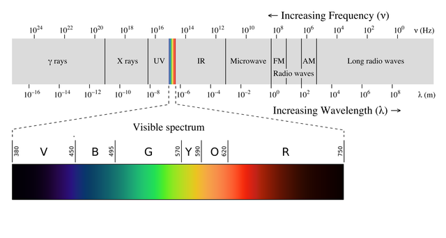
Infrared (IR) light is light that is of a lower frequency than visible light, while ultraviolet (UV) light is of a higher frequency than visible light.

When we think of light, we usually think of “visible light”, which is the only types of light that the human eye can see, but this is actually only a very small range of frequencies that light can have (see Figure 6).

For instance, bees and other insects can also see some ultraviolet frequencies, and many flowers have evolved quite unusual colour patterns which can only be detected by creatures that can see ultraviolet light – e.g., see here, here, or here. On the other hand, some animals, e.g., snakes, can see some infrared frequencies, which allows them to use “heat-sensing vision” to hunt their prey, e.g., see here or here.

As a simple rule of thumb, the hotter the object, the higher the frequencies of the light it emits. At room temperature, objects mostly emit light in the infrared region. However, when a coal fire gets hot enough, it also starts emitting light at higher frequencies, i.e., in the visible region. The coals become “red hot”.

Because the temperature at the surface of the Sun is nearly 6000 K, the light that it emits is mostly in the form of ultraviolet and visible (“UV-Vis.” for short), with some infrared light. In contrast, the surface of the Earth is only about 300 K, and so the light that the Earth emits is mostly low frequency infrared light (called “long infrared” or long-IR).

As the Sun shines light onto the Earth, this heats up the Earth’s surface and atmosphere. However, as the Earth’s surface and atmosphere heat up, they also emit more light. The average energy of the light reaching the Earth from the Sun, roughly matches the average energy of the light leaving the Earth into space. This works out at about 240 Watts per square metre of the Earth’s surface.

This brings us to the greenhouse effect theory.

In the 19th century, an Irish scientist named John Tyndall discovered that some of the gases in the Earth’s atmosphere interact with infrared light, but others don’t. Tyndall, 1861 (DOI; .pdf available here) showed that nitrogen (N₂) and oxygen (O₂) are totally transparent to infrared light. This was important because nitrogen and oxygen make up almost all of the gas in the atmosphere. The third most abundant gas in the atmosphere, argon (Ar) wasn’t discovered until several decades later, but it also is transparent to infrared light.

However, he found that some of the gases which only occurred in trace amounts (“trace gases”) do interact with infrared light. The main “infrared-active” gases in the Earth’s atmosphere are water vapour (H₂O), carbon dioxide (CO₂), ozone (O₃) and methane (CH₄).

Because the light leaving the Earth is mostly infrared light, some researchers suggested that these infrared-active gases might alter the rate at which the Earth cooled to space. This theory has become known as the “greenhouse effect” theory, and as a result, infrared-active gases such as water vapour and carbon dioxide are often referred to as “greenhouse gases”.

In this essay, we well stick to the more scientifically relevant term, infrared-active gases instead of the greenhouse gas term.

Greenhouse effect theory: “It’s simple physics” version

In crude terms, the greenhouse effect theory predicts that temperatures in the troposphere will be higher in the presence of infrared-active gases than they would be otherwise.

If the greenhouse effect theory were true then increasing the concentration of carbon dioxide in the atmosphere should increase the average temperature in the troposphere, because carbon dioxide is an infrared-active gas. That is, carbon dioxide should cause “global warming”.

This is the basis for the man-made global warming theory. The burning of fossil fuels releases carbon dioxide into the atmosphere. So, according to the man-made global warming theory, our fossil fuel usage should be warming the planet by “enhancing the greenhouse effect”.

Therefore, in order to check if man-made global warming theory is valid, it is important to check whether or not the greenhouse effect theory is valid. When we first started studying the greenhouse effect theory in detail, one of the trickiest things to figure out was exactly what the theory was supposed to be. We found lots of people who would make definitive claims, such as “it’s simple physics”, “it’s well understood”, or “they teach it in school, everyone knows about it…”:

Simple physics says, if you increase the concentration of carbon dioxide in the atmosphere, the temperature of the earth should respond and warm. – Prof. Robert Watson (Chair of the Intergovernmental Panel on Climate Change, 1997-2002) during a TV debate on global warming. 23rd November 2009

…That brings up the basic science of global warming, and I’m not going to spend a lot of time on this, because you know it well… Al Gore in his popular presentation on man-made global warming – An Inconvenient Truth (2006)

However, when pressed to elaborate on this allegedly “simple” physics, people often reverted to hand-waving, vague and self-contradictory explanations. To us, that’s not “simple physics”. Simple physics should be clear, intuitive and easy to test and verify.

At any rate, one typical explanation that is offered is that when sunlight reaches the Earth, the Earth is heated up, and that infrared-active gases somehow “trap” some of this heat in the atmosphere, preventing the Earth from fully cooling down.

For instance, that is the explanation used by Al Gore in his An Inconvenient Truth (2006) presentation:

The “heat-trapping” version of the greenhouse effect theory is promoted by everyone from environmentalist groups, e.g., Greenpeace, and WWF; to government websites, e.g., Australia, Canada and USA; and educational forums, e.g., Livescience.com, About.com, and HowStuffWorks.com.

However, despite its popularity, it is just plain wrong!

The Earth is continuously being heated by the light from the Sun, 24 hours a day, 365 days a year (366 in leap years). However, as we mentioned earlier, this incoming sunlight is balanced by the Earth cooling back into space – mainly by emitting infra-red light.

If infrared-active gases were genuinely “trapping” the heat from the sun, then every day the air would be continuously heating up. During the night, the air would continue to remain just as warm, since the heat was trapped. As a result, each day would be hotter than the day before it. Presumably, this would happen during the winter too. After all, because the sun also shines during the winter, the “trapped heat” surely would continue to accumulate the whole year round. Every season would be hotter than the one it followed. If this were true, then the air temperature would rapidly reach temperatures approaching that of the sun!

This is clearly nonsense – on average, winters tend to be colder than summers, and the night tends to be colder than the day.

It seems that the “simple physics” version of the greenhouse effect theory is actually just simplistic physics!

Having said that, this simplistic theory is not the greenhouse effect theory that is actually used by the current climate models. Instead, as we will discuss below, the “greenhouse effect” used in climate models is quite complex. It is also highly theoretical… and it has never been experimentally shown to exist.

In Sections 4-6, we will explain how our research shows that this more complicated greenhouse effect theory is also wrong. However, unlike the “simple physics” theory, it is at least plausible and worthy of investigation. So, let us now briefly summarise it…

Greenhouse effect theory: The version used by climate models

In the “simple physics” version of the greenhouse effect theory, infrared-active gases are supposed to “trap” heat in the atmosphere, because they can absorb infrared light.

As we discussed earlier, it is true that infrared-active gases such as water vapour and carbon dioxide can absorb infrared light. However, if a gas can absorb infrared light, it also can emit infrared light. So, once an infrared-active gas absorbs infrared light, it is only “trapped” for at most a few tenths of a second before it is re-emitted!

The notion that carbon dioxide “traps” heat might have made some sense in the 19th century, when scientists were only beginning to investigate heat and infrared light, but it is now a very outdated idea.

Indeed, if carbon dioxide were genuinely able to “trap” heat, then it would be such a good insulator, that we would use it for filling the gap in double-glazed windows. Instead, we typically use ordinary air because of its good insulation properties, or even use pure argon (an infrared-inactive gas), e.g., see here or here.

So, if carbon dioxide doesn’t trap heat, why do the current climate models still predict that there is a greenhouse effect?

Well, while infrared-active gases can absorb and emit infrared light, there is a slight delay between absorption and emission. This delay can range from a few milliseconds to a few tenths of a second.

The length of time between absorption and emission depends on the Einstein coefficients of the gas, which are named after the well-known physicist, Albert Einstein, for his research into the topic in the early 20th century.

This might not seem like much, but for that brief moment between absorbing infrared light and emitting it again, the infrared-active gas is more energetic than its neighbouring molecules. We say that the molecule is “excited”. Because the molecules in a gas are constantly moving about and colliding with each other, it is very likely that some nearby nitrogen or oxygen molecule will collide with our excited infrared-active gas molecule before it has a chance to emit its light.

During a molecular collision, molecules can exchange energy and so some of the excited energy ends up being transferred in the process. Since the infrared-inactive gases don’t emit infrared light, if enough absorbed energy is transferred to the nitrogen and oxygen molecules through collisions, that could theoretically increase the average energy of the air molecules, i.e., it could “heat up” the air.

It is this theoretical “collision-induced” heating effect that is the basis for the greenhouse effect actually used by the climate models, e.g., see Pierrehumbert, 2011 (Abstract; Google Scholar access).

Now, astute readers might be wondering about our earlier discussion on energy equilibrium. If the atmosphere is in energy equilibrium, then as soon as one part of the atmosphere starts gaining more energy than another, the atmosphere should start rapidly redistributing that energy, and thereby restoring energy equilibrium.

This means that any “energetic pockets” of air which might start to form from this theoretical greenhouse effect would immediately begin dissipating again. In other words, if the atmosphere is in energy equilibrium then the greenhouse effect cannot exist!

So, again, we’re back to the question of why the current climate models predict that there is a greenhouse effect.

The answer is simple. They explicitly assume that the atmosphere is not in energy equilibrium, but only in local energy equilibrium.

Is this assumption valid? Well, the people who developed the current climate models believe it is, but nobody seems to have ever checked if it was. So, in our three papers, we decided to check. In Sections 4-6, we will describe the resuls of that check. It turns out that the atmosphere is actually in complete energy equilibrium – at least over the distances of the tens of kilometres from the bottom of the troposphere to the top of the stratosphere.

In other words, the local energy equilibrium assumption of the current climate models is wrong.

Nonetheless, since the greenhouse effect theory is still widely assumed to be valid, it is worth studying its implications a little further, before we move onto our new research…

When we hear that carbon dioxide is supposed to increase the greenhouse effect, probably most of us would assume that the whole atmosphere is supposed to uniformly heat up. However, the proposed greenhouse effect used by the models is actually quite complicated, and it varies dramatically throughout the atmosphere.

There are several reasons for this.

Although the rate of infrared absorption doesn’t depend on the temperature of the infrared-active gases, the rate of emission does. The hotter the molecules, the more infrared light it will emit. However, when a gas molecule emits infrared light, it doesn’t care what direction it is emitting in! According to the models, this means that when the air temperature increases, the rate at which infrared light is emitted into space increases, but so does the rate at which infrared light heads back to ground (“back radiation”).

Another factor is that, as you go up in the atmosphere, the air gets less dense. This means that the average length of time between collisions amongst the air molecules will increase. In other words, it is more likely that excited infrared-active gas molecules will be able to stay excited long enough to emit infrared light.

Finally, the infrared-active gases are not uniformly distributed throughout the atmosphere. For instance, the concentration of water vapour decreases rapidly above the boundary layer, and is higher in the tropics than at the poles. Ozone is another example in that it is mostly found in the mid-stratosphere in the so-called “ozone layer” (which we will discuss below).

With all this in mind, we can see that it is actually quite a difficult job to calculate exactly what the “greenhouse effect” should be at each of the different spots in the atmosphere. According to the theory, the exact effect will vary with height, temperature, latitude and atmospheric composition.

Climate modellers refer to the various attempts at these calculations as “infrared cooling models”, and researchers have been proposing different ones since the 1960s, e.g., Stone & Manabe, 1968 (Open access).

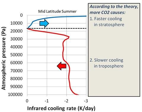
Deciding which infrared cooling model to include in the climate models has been the subject of considerable debate over the years. It has been a particularly tricky debate, because nobody has ever managed to experimentally measure an actual infrared cooling profile for the atmosphere. Nonetheless, most of the ones used in the current climate models are broadly similar to the one in Figure 8.

We can see that these models predict that infrared-active gases should slow down the rate of infrared cooling in the troposphere. This would allow the troposphere to stay a bit warmer, i.e., cause global warming. However, as you go up in the atmosphere, two things happen:

1. The density of the air decreases. This means that when an infrared-active gas emits infrared light, it is more likely to “escape” to space.
2. The average temperature of the air increases in the stratosphere. This means the rate of infrared emission should increase.

For these two reasons, the current climate models predict that increasing infrared-active gases should actually speed up the rate at which the tropopause and stratosphere cool. So, the calculated “global warming” in the troposphere is at the expense of “global cooling” in the stratosphere, e.g., Hu & Tung, 2002 (Open access) or Santer et al., 2003 (Abstract; Google Scholar access).

Why do temperatures (a) stop decreasing with height in the tropopause, and (b) start increasing with height in the stratosphere?

According to the current climate models, it is pretty much all due to the ozone layer.

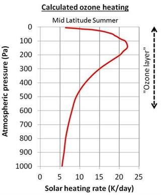
When sunlight reaches the planet, the light includes a wide range of frequencies – from infrared light through visible light to ultraviolet light. However, when the sunlight reaches us at the ground, most of the high frequency ultraviolet light has been absorbed. This is because the ozone in the ozone layer absorbs it.

The fact that the ozone layer absorbs ultraviolet light is great for us, because high frequency ultraviolet light is very harmful to most organisms. Life as we know it probably couldn’t exist in the daylight, if all of the sun’s ultraviolet light reached us.

Anyway, because the models assume the atmosphere is only in local energy equilibrium, they conclude that when the ozone absorbs the ultraviolet light, it heats up the air in the ozone layer.

As the light passes through the atmosphere, there is less and less ultraviolet light to absorb, and so the amount of “ozone heating” decreases (Figure 9). The concentration of ozone also decreases once you leave the ozone layer.

So, according to the climate models, the reason why temperatures increase with height in the stratosphere is because of ozone heating. In the tropopause, there is less ozone heating, but they reckon there is still enough to counteract the normal “gravitational cooling”, and that’s why the temperature “pauses”, i.e., remains constant with height.

As we discuss in Paper I, there are major problems with this theory.

First, it relies on the assumption that the atmosphere is only in local energy equilibrium, which has never been proven.

Second, it implies that the tropopause and stratosphere wouldn’t occur without sunlight. During the winter at the poles, it is almost pitch black for several months, yet the tropopause doesn’t disappear. In other words, the tropopause does not need sunlight to occur. Indeed, if we look back at Figure 2, we can see that the tropopause is actually more pronounced for the poles, in that it starts at a much lower height than it does at lower latitudes.

In Section 5, we will put forward a more satisfactory explanation.

Has anyone ever measured the greenhouse effect?

Surprisingly, nobody seems to have actually observed this alleged greenhouse effect … or the ozone heating effect, either!

The theory is based on a few experimental observations:

1. As we discussed earlier, all objects, including the Earth, can cool by emitting light. Because the Earth only has a temperature of about 300K, this “cooling” light is mostly in the form of infrared light.
2. The main gases in the atmosphere (i.e., nitrogen, oxygen and argon) can’t directly absorb or emit infrared light, but the infrared-active gases (e.g., water vapour, carbon dioxide, ozone and methane) can.
3. Fossil fuel usage releases carbon dioxide into the atmosphere, and the concentration of carbon dioxide in the atmosphere has been steadily increasing since at least the 1950s (from 0.031% in 1959 to 0.040% in 2013).

We don’t disagree with these observations. But, they do not prove that there is a greenhouse effect.

The greenhouse effect theory explicitly relies on the assumption that the atmosphere is in local energy equilibrium, yet until we carried out our research, nobody seems to have actually experimentally tested if that assumption was valid. If the assumption is invalid (as our results imply), then the theory is also invalid.

Even aside from that, the greenhouse effect theory makes fairly specific theoretical predictions about how the rates of “infrared cooling” and “ozone heating” are supposed to vary with height, latitude, and season, e.g., Figures 8 and 9. Yet, nobody seems to have attempted to experimentally test these theoretical infrared cooling models, either.

Of course, just because a theory hasn’t been experimentally tested, that doesn’t necessarily mean it’s wrong. However, it doesn’t mean it’s right, either!

With that in mind, we felt it was important to physically check what the data itself was saying, rather than presuming the greenhouse effect theory was right or presuming it was wrong… After all, “Nature” doesn’t care what theories we happen to believe in – it just does its own thing!

Some researchers have claimed that they have “observed” the greenhouse effect, because when they look at the infrared spectrum of the Earth’s atmosphere from space they find peaks due to carbon dioxide, e.g., Harries et al., 2001 (Abstract; Google Scholar access). However, as we discuss in Section 3.2 of Paper II, that does not prove that the greenhouse effect exists. Instead, it just shows that it is possible to use infrared spectroscopy to tell us something about the atmospheric composition of planets.

Paper 1: Phase change associated with tropopause

We suspected that the change in temperature behaviour at the tropopause was actually related to a change in the molecular properties of the air. So, we decided to analyse weather balloon data in terms of a molecular property known as the “molar density”. The molar density of a gas tells you the average number of molecules per cubic metre of the gas. Since there are a LOT of molecules in a cubic metre of gas, it is expressed in terms of the number of “moles” of gas per cubic metre. One mole of a substance corresponds to about 600,000,000,000,000,000,000,000 molecules, which is quite a large number!

We downloaded weather balloon data for the entire North America continent from the University of Wyoming archive. We then used this data to calculate the change in molar density with pressure.

Atmospheric pressure decreases with height (altitude), and in space, the atmospheric pressure is almost zero. Similarly, molar density decreases with height, and in space, is almost zero. So, in general, we would expect molar density to decrease as the pressure decreases. This is what we found. However, there were several surprising results.

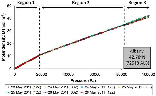
Figure 10 shows the molar density plots calculated from the measurements of seven different weather balloons launched over a period of 4 days from Albany, New York (USA) in May 2011.

Since atmospheric pressure decreases as we go up in the atmosphere, in these plots, the balloon height increases as we go from right to left. That is, the ground level corresponds to the right hand side of the plot and the left hand side corresponds to the upper atmosphere. The three different regions are discussed in the text below.

There are several important things to note about these plots:

• The measurements from all seven of the weather balloons show the same three atmospheric regions (labelled Regions 1-3 in the figure).
• For Regions 1 and 2, the molar density plots calculated from all of the balloons are almost identical, i.e., the dots from all seven balloons fall on top of each other.
• In contrast, the behaviour of Region 3 does change a bit from balloon to balloon, i.e., the dots from the different balloons don’t always overlap.
• The transition between Regions 1 and 2 corresponds to the transition between the troposphere and the tropopause. This suggests that something unusual is happening to the air at the start of the tropopause.
• There is no change in behaviour between the tropopause and the stratosphere, i.e., when you look at Region 1, you can’t easily tell when the tropopause “ends” and when the stratosphere “begins”. This suggests that the tropopause and stratosphere regions are not two separate “regions”, but are actually both part of the same region.

When we analysed the atmospheric water concentration measurements for the balloons, we found that the different slopes in Region 3 depended on how humid the air in the region was, and whether or not the balloon was travelling through any clouds or rain.

On this basis, we suggest that the Region 3 variations are mostly water-related. Indeed, Region 3 corresponds to the boundary layer part of the troposphere, which is generally the wettest part of the atmosphere.

What about Regions 1 and 2? The change in behaviour of the plots between Regions 1 and 2 is so pronounced that it suggests that some major change in the atmosphere occurs at this point.

In Paper 2, we propose that this change is due to some of the oxygen and/or nitrogen in the air joining together to form molecular “clusters” or “multimers”. We will discuss this theory in Section 5.

For now, it is sufficient to note that the troposphere-tropopause transition corresponds to some sort of “phase change”. In Paper 1, we refer to the air in the troposphere as being in the “light phase”, and the air in the tropopause/stratosphere regions being in the “heavy phase”

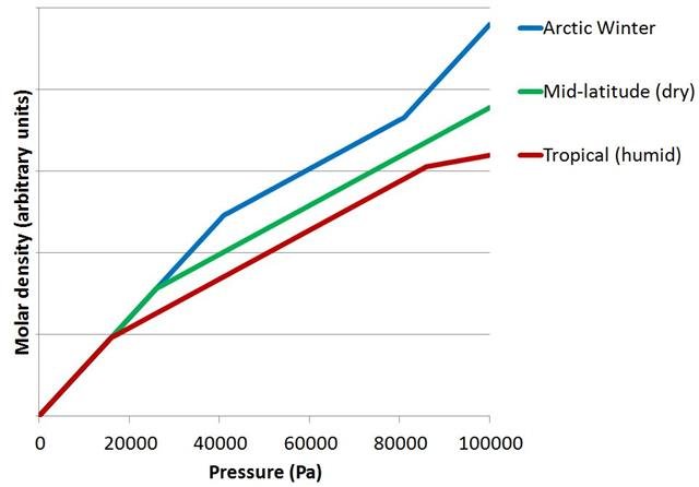
When we analyse weather balloon measurements from other locations (and seasons), the same general features occur.

However, there are some differences, which we illustrate schematically in Figure 11. In tropical locations, the heavy phase/light phase transition occurs much higher in the atmosphere (i.e., at a lower pressure). In contrast, in the Arctic, the heavy phase/light phase change occurs much lower in the atmosphere (i.e., at a higher pressure). This is in keeping with the fact that the height of the tropopause is much higher in the tropics than at the poles (as we saw in Figure 2).

One thing that is remarkably consistent for all of the weather balloon measurements we analysed is that in each of the regions, the change of molar density with pressure is very linear. Another thing is that the change in slope of the lines between Regions 1 and 2 is very sharp and distinct.

Interestingly, on very cold days in the Arctic winter, we often find the slopes of the molar density plots near ground level (i.e., Region 3) are similar to the slope of the “heavy phase” (schematically illustrated in Figure 11).

The air at ground level is very dry under these conditions, because it is so cold. So, this is unlikely to be a water-related phenomenon. Instead, we suggest that it is because the temperatures at ground level in the Arctic winter are cold enough to cause something similar to the phase change which occurs at the tropopause.

At this stage you might be thinking: “Well, that’s interesting what you discovered… But, what does this have to do with the temperature profiles?”

Well, since we calculated the molar densities from the temperature and pressure measurements of the balloons, we can also convert molar densities back into temperature values. Since we found that the relationship between molar density and pressure was almost linear in each region, we decided to calculate what the temperatures would be if the relationship was exactly linear. For the measurements of each weather balloon, we calculated the best linear fit for each of the regions (using a statistical technique known as “ordinary least squares linear regression”). We then converted these linear fits back into temperature estimates for each of the pressures measured by the balloons.

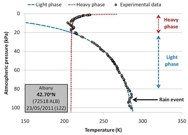
In Figure 12, we compare the original balloon measurements for one of the Albany, New York balloons to our linear fitted estimates.

Because pressure decreases with height, we have arranged the graphs in this essay so that the lowest pressures (i.e., the stratosphere) are at the top and the highest pressures (i.e., ground level) are at the bottom.

The black dots correspond to the actual balloon measurements, while the two dashed lines correspond to the two temperature fits.

We find the fits to be remarkable. Aside from some deviations in the boundary layer (at around 90kPa) which are associated with a rain event, the measurements fall almost exactly onto the blue “light phase” curve all the way up to the tropopause, i.e., 20kPa. In the tropopause and stratosphere, the measurements fall almost exactly onto the red “heavy phase” curve.

We found similar strong fits to all of the balloons we applied this approach to. The exact values we used for the fits varied from balloon to balloon, but in all cases the balloon measurements could be fit using just two (or sometimes three) phases.

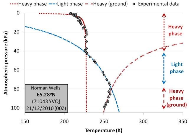
Examples of the balloons which needed to be fitted with three phases were those launched during the winter in the Arctic region. For instance, Figure 13 shows the balloon measurements and fits for a balloon launched from Norman Wells, Northwest Territories (Canada) in December 2010.

Again, the matches between the experimental data and our linear fits are very good.

For these balloons, the slope of the molar density plots for the region near the ground level (Region 3) is very similar to the slope of the heavy phase in Region 1. This is in keeping with our earlier suggestion that the air near ground level for these cold Arctic winter conditions is indeed in the heavy phase.

For us, one of the most fascinating findings of this analysis is that the atmospheric temperature profiles from the boundary layer to the middle of the stratosphere can be so well described in terms of just two or three distinct regions, each of which has an almost linear relationship between molar density and pressure.

The temperature fits did not require any consideration of the concentration of carbon dioxide, ozone or any of the other infrared-active gases. This directly contradicts the greenhouse effect theory, which claims that the various infrared-active gases dramatically alter the atmospheric temperature profile.

As we saw in Section 3, the greenhouse effect theory predicts that infrared-active gases lead to complicated infrared cooling rates which should be different at each height (e.g., the one in Figure 9). According to the theory, infrared-active gases partition the energy in the atmosphere in such a way that the atmospheric energy at each height is different.

This means that we should be finding a very complex temperature profile, which is strongly dependent on the infrared-active gases. Instead, we found the temperature profile was completely independent of the infrared-active gases.

This is quite a shocking result. The man-made global warming theory assumes that increasing carbon dioxide (CO₂) concentrations will cause global warming by increasing the greenhouse effect. So, if there is no greenhouse effect, this also disproves the man-made global warming theory.

Paper 2: Multimerization of atmospheric gases above the troposphere

In Paper 2, we decided to investigate what could be responsible for the phase change we identified in Paper 1. We suggest that it is due to the partial “multimerization” of oxygen and/or nitrogen molecules in the atmosphere above the troposphere. We will explain what we mean by this later, but first, we felt it was important to find out more information about how the conditions for this phase change vary with latitude and season.

Variation of phase change conditions

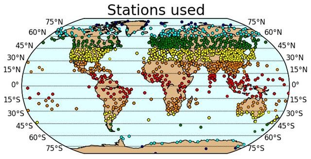
We downloaded weather balloon data from the Integrated Global Radiosonde Archive (IGRA) which is maintained by the NOAA National Climatic Data Center. The IGRA dataset contains weather balloon records from 1,109 weather stations located on all the continents – see Figure 14.

As each of the weather stations launches between 1 and 4 balloons per day, and has an average of about 36 years worth of data, this makes for a lot of data. To analyse all this data, we wrote a number of computer scripts, using the Python programming language.

Our scripts systematically analysed all of the available weather balloon records to identify the pressure and temperature at which the phase change occurred, i.e., the transition between Region 1 and Region 2.

If there wasn’t enough data for our script to calculate the change point, we skipped that balloon, e.g., some of the balloons burst before reaching the stratosphere. However, we were able to identify the transition for most of the balloons.

Below are the plots for all of the weather balloons launched in 2012 from one of the stations – Valentia Observatory, Ireland. The black dashed lines correspond to the phase change for that balloon.

In all, our scripts identified the phase change conditions for more than 13 million weather balloons.

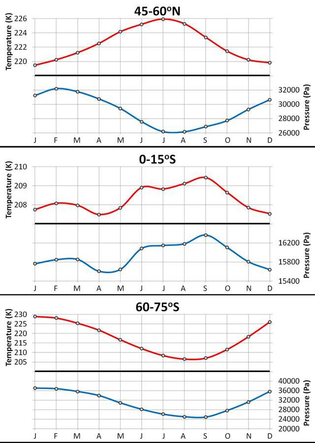
We decided to group the stations into twelve different latitudinal bands (see Figure 14). Then, for each of the bands, we calculated the average phase conditions for each month. Figure 15 shows the seasonal variations for three of the twelve latitudinal bands.

In Paper 2, we present the data for all twelve bands, and discuss the main features of the seasonal changes in some detail. However, for the purpose of this essay, it is sufficient to note the following features:

• Each latitudinal band has different patterns.
• All bands have very well defined annual cycles, i.e., every year the phase change conditions for each band goes through clear seasonal cycles.
• For some areas, and at some times of the year, the temperature and pressure conditions change in sync with each other, i.e., they both increase and decrease at the same time. At other times and places, the temperature and pressure changes are out of sync with each other.

In Section 4, we saw that the phase change conditions are directly related to the atmospheric temperature profiles.

This means that if we can figure out the exact reasons why the phase change conditions vary as they do with season and latitude, this should also provide us with insight into entire temperature profiles.

If we could do this, this could help meteorologists to make dramatically better weather predictions. So, in our paper, we discuss several interesting ideas for future research into understanding how and why the phase change conditions vary.

Multimerization of the air

At any rate, it seems likely to us that some major and abrupt change in the atmospheric composition and/or molecular structure is occurring at the tropopause.

However, measurements of the atmospheric composition don’t show any major change associated with the troposphere/tropopause transition. Both above and below the phase change, the atmosphere is 78% nitrogen, 21% oxygen and 1% argon.

Instead, we suggest that the phase change involves a change in the molecular structure of at least some of the air molecules. Although argon might be involved, it only comprises 1% of the atmosphere, so we will focus here on the oxygen and nitrogen molecules, which make up 99% of the atmosphere near the phase change.

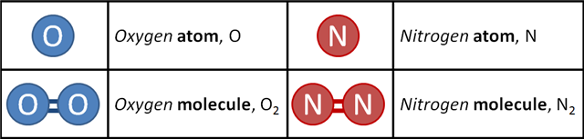
As can be seen in Figure 16, oxygen and nitrogen molecules are both “diatomic”, i.e., each molecule contains two atoms.

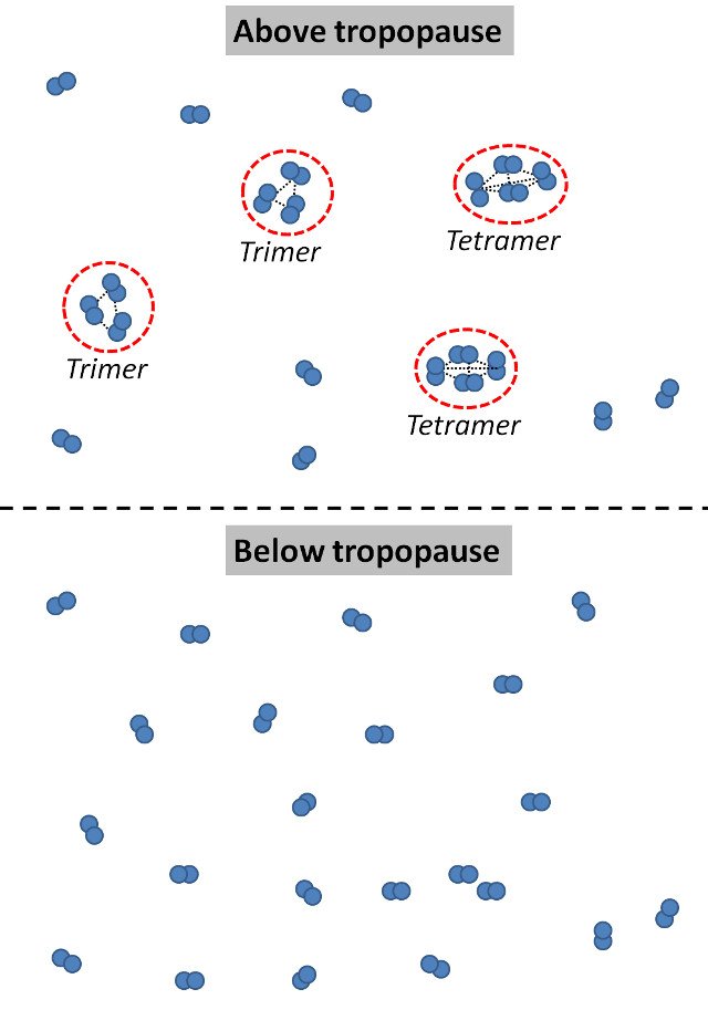
We suggest that, once the phase change conditions occur, some of these diatomic molecules begin clustering together to form “molecular clusters” or “multimers”. We illustrate this schematically in Figure 17.

Below the tropopause, all of the oxygen is the conventional diatomic oxygen that people are familiar with. Similarly, all of the nitrogen is diatomic. However, above the tropopause, some of these air molecules coalesce into large multimers.

Multimers take up less space per molecule than monomers. This reduces the molar density of the air. This explains why the molar density decreases more rapidly in Region 1 than in Region 2 (e.g., Figure 10).

It also has several other interesting implications…

Why temperature increases with height in the stratosphere

The current explanation for why temperatures stay constant with height in the tropopause and increase with height in the stratosphere is that ozone heats up the air in the ozone layer by absorbing ultraviolet light. However, as we discussed in Section 3, there are major problems with this explanation.

Fortunately, multimerization offers an explanation which better fits the data. We saw in Section 4 that the temperature behaviour in both the tropopause and stratosphere is very well described by our linear molar density fit for the “heavy phase” (have a look back at Figures 12 and 13, in case you’ve forgotten).

This suggests that the changes in temperature behaviour above the troposphere are a direct result of the phase change. So, if the phase change is due to multimerization, as we suggest, then the change in temperature behaviour is a consequence of multimerization.

Why would multimerization cause the temperature to increase with height?

Do you remember from Section 3 how we were saying there are four different types of energy that the air molecules have, i.e., thermal, latent, potential and kinetic?

Well, in general, the amount of energy that a molecule can store as latent energy decreases as the molecule gets bigger.

This means that when oxygen and/or nitrogen molecules join together to form larger multimer molecules, the average amount of latent energy they can store will decrease.

However, due to the law of conservation of energy, the total energy of the molecules has to remain constant. So, as we discussed in Section 3, if the latent energy of the molecules has to decrease, one of the other types of energy must increase to compensate.

In this case, the average thermal energy of the molecules increases, i.e., the temperature increases!

Changes in the ozone layer

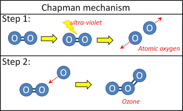
The conventional explanation for how ozone is formed in the ozone layer is the Chapman mechanism, named after Sydney Chapman who proposed it in 1930.

Ozone is an oxygen compound just like the oxygen molecules. Except, unlike regular diatomic oxygen, ozone is triatomic (O₃). This is quite an unusual structure to form, and when the ozone layer was discovered, scientists couldn’t figure out how and why it formed there.

Chapman suggested that ultraviolet light would occasionally be powerful enough to overcome the chemical bond in an oxygen molecule, and split the diatomic molecule into two oxygen atoms.

Oxygen atoms are very unstable. So, Chapman proposed that as soon as one of these oxygen atoms (“free radicals”) collided with an ordinary diatomic oxygen molecule, they would react together to form a single triatomic ozone molecule (Figure 18).

This Chapman mechanism would require a lot of energy to take place, and so it was assumed that it would take several months for the ozone layer to form. But, nobody was able to come up with an alternative mechanism that could explain the ozone layer.

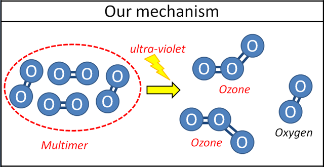
However, if multimerization is occurring in the tropopause/stratosphere, then this opens up an alternative mechanism.

We suggest that most of the ozone in the ozone layer is actually formed by the splitting up of oxygen multimers! We illustrate this mechanism in the schematic in Figure 19.

As in the Chapman mechanism, ultraviolet light can sometimes provide enough energy to break chemical bonds. However, because there are a lot more oxygen atoms in an oxygen multimer than in a regular diatomic oxygen molecule, the ultraviolet light doesn’t have to split the oxygen into individual atoms. Instead, it can split the multimer directly into ozone and oxygen molecules. This doesn’t require as much energy.

To test this theory, we decided to see if there was any relationship between the concentration of ozone in the ozone layer, and the phase change conditions.

We downloaded from the NASA Goddard Space Flight Center’s website all of the available monthly averaged ozone measurements from the NASA Total Ozone Mapping Spectrometer (TOMS) satellite (August 1996-November 2005). We then averaged together the monthly values for the same twelve latitudinal band we used for our weather balloons.

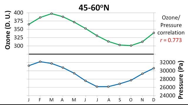
When we compared the seasonal variations in ozone concentrations for each band to the seasonal variations in the phase change conditions, we found they were both highly correlated! For instance, Figure 20 compares the average monthly pressure of the phase change to the average monthly ozone concentrations for the 45-60°N band.

If ozone was been mainly formed by the conventional Chapman mechanism, then there is no reason why the ozone concentrations should be correlated to the phase change conditions. However, if the ozone is being formed by our proposed mechanism, then it makes sense.

To us this indicates that most of the ozone in the ozone layer is formed from oxygen multimers, and not by the Chapman mechanism, as has been assumed until now.

It also suggests that we have seriously underestimated the rates at which the ozone layer expands and contracts. Figure 20 shows how the thickness of the ozone layer is strongly correlated to the phase change conditions.

But, these phase change conditions change dramatically from month to month. This means that ozone is formed and destroyed in less than a month. This is much quicker than had been previously believed.

New explanation for the jet streams

When we wrote our scripts to analyse the temperatures and pressures of the phase change conditions, we also looked at the average wind speeds measured by the weather balloons. You might have noticed in the video we showed earlier of the Valentia Observatory phase changes for 2012 that the bottom panels showed the average wind speeds recorded by each balloon.

We noticed an interesting phenomenon. At a lot of weather stations, very high wind speeds often occurred near the phase change. When the pressure at which the phase change occurred increased or decreased, the location of these high wind speeds would also rise or fall in parallel.

This suggested to us that the two phenomena were related. So, we decided to investigate. On closer inspection, we noticed that the weather stations we were detecting high wind speeds for were located in parts of the world where the jet streams occur.

The jet streams are narrow bands of the atmosphere near the tropopause in which winds blow rapidly in a roughly west to east direction (Figure 21). It turns out that the high wind speeds we were detecting were the jet streams!

But, these high winds seemed to be strongly correlated to the phase change conditions. This suggested to us that multimerization might be involved in the formation of the jet streams.

Why should multimerization cause high wind speeds?

Well, as we mentioned earlier, when multimers form they take up less space than regular air molecules, i.e., the molar density decreases.

So, if multimers rapidly form in one part of the atmosphere, the average molar density will rapidly decrease. This would reduce the air pressure. In effect, it would form a partial “vacuum”. This would cause the surrounding air to rush in to bring the air pressure back to normal. In other words, it would generate an inward wind.

Similarly, if multimers rapidly break down, the average molar density will rapidly increase, causing the air to rush out to the sides. That is, it would generate an outward wind.

We suggest that the jet streams form in regions where the amount of multimerization is rapidly increasing or decreasing.

New explanation for tropical cyclones

Our analysis also offers a new explanation for why tropical cyclones (hurricanes, typhoons, etc.) form. Tropical cyclones form and exist in regions where there is no jet stream.

We suggest cyclones occur when the “vacuum” formed by multimerization is filled by “sucking” air up from below, rather than sucking from the sides as happens with the jet streams. This reduces the atmospheric pressure at sea level, leading to what is known as “cyclonic behaviour”.

Similarly, if the amount of multimers rapidly decreases, this can “push” the air downwards leading to an increase in the atmospheric pressure at sea level, causing “anti-cyclonic behaviour”.

Meteorologists use the term “cyclone” to refer to any low-pressure system, not just the more dangerous tropical cyclones. But, if an ordinary cyclone forms over a warm ocean, then the cyclone can suck up some of the warm water high into the atmosphere. This water freezes when it gets up high, releasing energy, and making the cyclone even stronger.

It is this extra energy released from the warm water freezing which turns an ordinary cyclone into a powerful tropical cyclone. This was already known for the standard explanation for how tropical cyclones are formed, e.g., see here.

However, until now, it had been assumed that tropical cyclones were formed at sea level. We suggest that the initial cyclone which leads to the more powerful tropical cyclone is actually formed much higher, i.e., at the tropopause, and that it is a result of multimerization.

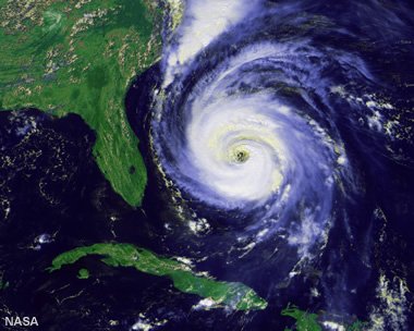
By the way, when water is drained down a sink hole, it often leaves in a whirlpool pattern. In the same way, if multimerization causes air to be sucked up to the tropopause from the surface, it might be sucked up in a whirlpool manner. This explains why if you look at satellite photographs for the cloud structures of tropical cyclones, they usually have a whirlpool-like structure, as in Figure 22.

We hope that this new way of looking at tropical cyclones will allow meteorologists to make better and more accurate predictions of hurricanes, typhoons and other tropical cyclones.

It might also help us to better understand why high pressure and low pressure weather systems (Figure 23) develop and dissipate. Much of the day-to-day job of meteorologists involves interpreting and predicting how these weather systems vary from day to day, and hour to hour. So, if rapid changes in the phase change conditions play a role in forming high and low pressure areas, then studying this could provide us with more accurate weather predictions.

Paper 3: Pervective power

In Section 3, we explained that a fundamental assumption of the greenhouse effect theory is that the atmosphere is only in local energy equilibrium. But, our results in Papers 1 and 2 suggested that the atmosphere were effectively in complete energy equilibrium – at least over the distances from the bottom of the troposphere to the top of the stratosphere. Otherwise, we wouldn’t have been able to fit the temperature profiles with just two or three parameters.

If the atmosphere is in energy equilibrium, then this would explain why the greenhouse effect theory doesn’t work.

However, when we consider the conventional energy transmission mechanisms usually assumed to be possible, they are just not fast enough to keep the atmosphere in complete energy equilibrium.

So, in Paper 3, we decided to see if there might be some other energy transmission mechanism which had been overlooked. Indeed, it turns out that there is such a mechanism. As we will see below, it seems to be rapid enough to keep the atmosphere in complete energy equilibrium over distances of hundreds of kilometres. In other words, it can explain why the greenhouse effect theory is wrong!

We call this previously unidentified energy transmission mechanism “pervection”, to contrast it with convection.

There are three conventional energy transmission mechanisms that are usually considered in atmospheric physics:

1. Radiation
2. Convection
3. Conduction

Radiation is the name used to describe energy transmission via light. Light can travel through a vacuum, and doesn’t need a mass to travel, e.g., the sunlight reaching the Earth travels through space from the Sun.

However, the other two mechanisms need a mass in order to work.

In convection, energy is transported by mass transfer. When energetic particles are transported from one place to another, the particles bring their extra energy with them, i.e., the energy is transported with the travelling particles. This is convection.

There are different types of convection, depending on the types of energy the moving particles have. If the moving particles have a lot of thermal energy, then this is called thermal convection. If you turn on an electric heater in a cold room, most of the heat will move around the room by thermal convection.

Similarly, if the moving particles have a lot of kinetic energy, this is called kinetic convection. When a strong wind blows, this transfers a lot of energy, even if the wind is at the same temperature as the rest of the air.

You can also have latent convection, e.g., when water evaporates or condenses to form clouds and/or precipitation, this can transfer latent energy from one part of the atmosphere to another.

Conduction is a different mechanism in that energy can be transmitted through a mass without the mass itself moving. If a substance is a good conductor, then it can rapidly transfer thermal energy from one side of the substance to another.

If one side of a substance is hotter than the other, then conduction can redistribute the thermal energy, so that all of the substance reaches the same temperature. However, conduction is only able to transfer thermal energy.

You can also have electrical conduction, in which electricity is transmitted through a mass.

Since air is quite a poor conductor, conduction is not a particularly important energy transmission mechanism for the atmosphere.

For this reason, the current climate models only consider convection and radiation for describing energy transport in the atmosphere. But, could there be another energy transmission mechanism the models are leaving out?

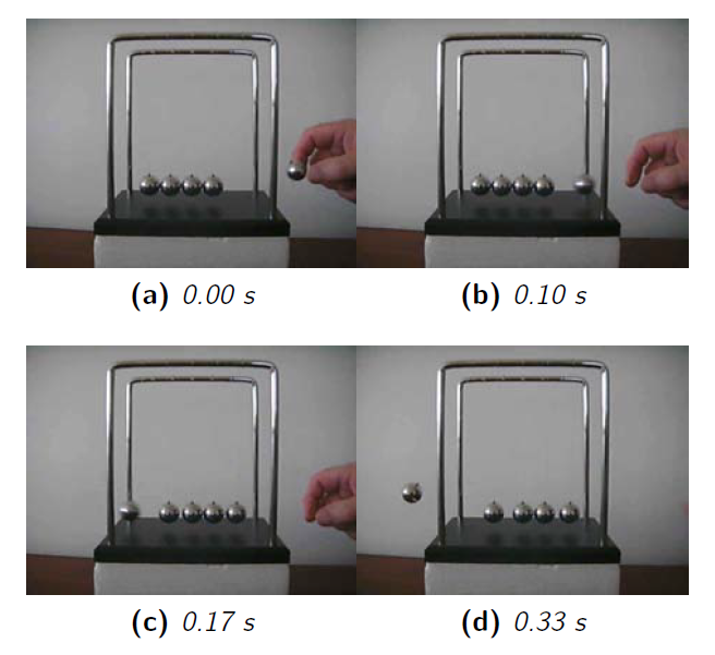
We realised there was. Consider the Newton’s cradle shown in Figure 24.

When you lift the ball on the left into the air and release it, you are providing it with mechanical energy, which causes it to rapidly swing back to the other balls.

When it hits the other balls, it transfers that energy on. But, then it stops. After a very brief moment, the ball on the other side of the cradle gets that energy, and it flies up out of the cradle.

Clearly, energy has been transmitted from one side of the cradle to the other. However, it wasn’t transmitted by convection, because the ball which originally had the extra energy stopped once it hit the other balls.

It wasn’t conduction, either, because the energy that was being transmitted was mechanical energy, not thermal energy.

In other words, mechanical energy can be transmitted through a mass. This mechanism for energy transmission is not considered in the current climate models. This is the mechanism that we call pervection.

Since nobody seems to have considered this mechanism before, we decided to carry out laboratory experiments to try and measure how quickly energy could be transmitted through air by pervection.

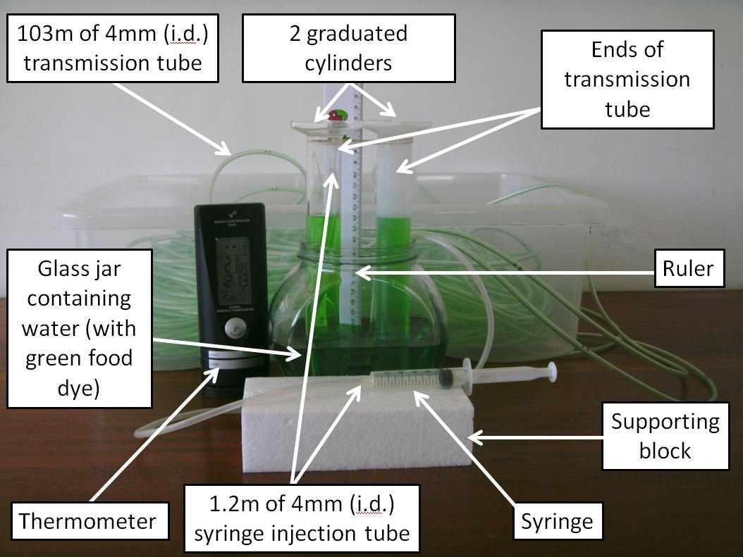
Figure 25 shows the experimental setup we used for these experiments.

In our experiment we connected two graduated cylinders with a narrow air tube that was roughly 100m long. We then placed the two cylinders upside down in water (which we had coloured green to make it easier to see). We also put a second air tube into the graduated cylinder on the left, and we used this tube to suck some of the air out of the cylinders. This raised the water levels to the heights shown in Figure 25. Then we connected the second tube to a syringe.

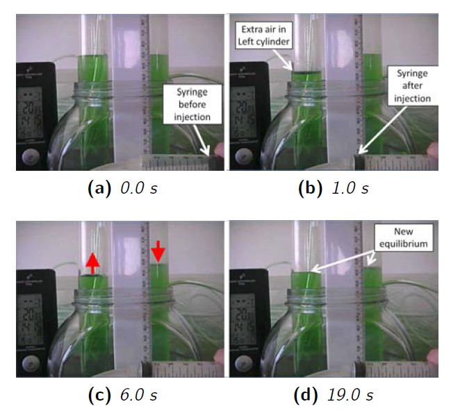
Figure 26 shows the basic idea behind the experiment. We used the syringe to push a volume of air into the air gap at the top of the cylinder on the left.

This caused the air gap in the left cylinder to expand, pushing the water level down, i.e., it increased the mechanical energy of the air in the air gap. However, over the next 10-20 seconds, two things happened. The water level in the left cylinder started rising again and the water level in the cylinder on the right started to fall.

19 seconds after the initial injection, the water levels in both sides had stopped moving, and had reached a new equilibrium.

There are several interesting points to note about this:

• Some of the mechanical energy transferred to the cylinder on the left was transmitted to the cylinder on the right
• This energy transmission was not instantaneous
• But, it was quite fast, i.e., it had finished after 19 seconds

What does this mean? Well, mechanical energy was somehow transmitted from the cylinder on the left to the one on the right.

This energy was transmitted through the air in the 100m tube that connects the two cylinders.

Since we are looking at energy transmission through air, we are considering the same energy transmission mechanisms that apply to the atmosphere.

Could the energy have been transmitted by conduction? No. First, it was mechanical energy which was transmitted, not thermal energy. And second, air is too poor a conductor.

Could the energy have been transmitted by radiation? No. Again, radiation is a mechanism for transmitting thermal energy, not mechanical energy. But in addition, radiation travels in straight lines. If you look at the setup in Figure 25, you can see that we had wrapped the 100m air tube in multiple loops in order to fit it into a storage box. So, the energy wouldn’t be able to travel all the way down the tube by radiation.

The only remaining conventional energy transmission mechanism is convection. However, the air was moving far too slowly for the energy to reach the cylinder on the right by the air being physically moved from one cylinder to the other.

When we calculated the maximum speed the air could have been moving through the 100m tube, it turned out that it would take more than an hour for the energy to be transmitted by convection. Since the energy transmission took less than 19 seconds, it wasn’t by convection!

That leaves pervection.

In the experiment shown, the left and right cylinders were physically close to each other, so maybe you might suggest that the energy was transmitted directly from one cylinder to the other by radiation, due to their close proximity. However, we obtained the same results when we carried out similar experiments where the two cylinders were placed far apart.

You can watch the video of our experiment below. The experiment is 5 minutes long, and consists of five cycles. We alternated between pushing and pulling the syringe every 30 seconds.

In the paper, we estimate that pervection might be able to transmit energy at speeds close to 40 metres per second.

Since the distance from the bottom of the troposphere to the top of the stratosphere is only about 50 km, that means it should only take about 20 minutes for energy to be transmitted between the troposphere and stratosphere. This should be fast enough to keep the troposphere, tropopause and stratosphere in complete energy equilibrium, i.e., it explains why the greenhouse effect theory doesn’t work.

Applying the scientific method to the greenhouse effect theory

If a physical theory is to be of any practical use, then it should be able to make physical predictions that can be experimentally tested. After all, if none of the theory’s predictions can actually be tested, then what is the point? The late science philosopher, Dr. Karl Popper described this as the concept of “falsifiability”. He reckoned that, for a theory to be scientific, it must be possible to construct an experiment which could potentially disprove the theory.

There seems to be a popular perception that the greenhouse effect and man-made global warming theories cannot be tested because “we only have one Earth”, and so, unless we use computer models, we cannot test what the Earth would be like if it had a different history of infrared-active gas concentrations. For instance, the 2007 IPCC reports argue that:

“A characteristic of Earth sciences is that Earth scientists are unable to perform controlled experiments on the planet as a whole and then observe the results.” – IPCC, Working Group 1, 4th Assessment Report, Section 1.2

To us, this seems a defeatist approach – it means saying that those theories are non-falsifiable, and can’t be tested. This is simply not true. As we said above, if a physical theory is to be of any use, then it should be able to make testable physical predictions. And by predictions, we mean “predictions” on what is happening now. If a scientist can’t test their predictions for decades or even centuries, then that’s a long time to be sitting around with nothing to do!

Instead, a scientist should use their theories to make predictions about what the results of experiments will be, and then carry out those experiments. So, we wondered what physical predictions the greenhouse effect theory implied, which could be tested… now! It turns out that there are fundamental predictions and assumptions of the theory which can be tested.

For instance, we saw in Section 3 that the theory predicts that the temperatures of the atmosphere at each altitude are related to the amount of infrared-active gases at that altitude. It also predicts that the greenhouse effect partitions the energy in the atmosphere in such a way that temperatures in the troposphere are warmer than they would be otherwise, and temperatures above the troposphere are colder than they would be otherwise.

However, our new approach shows that this is not happening! In Paper 1, we showed that the actual temperature profiles can be simply described in terms of just two or three linear regimes (in terms of molar density). In Paper 2, we proposed a mechanism to explain why there is more than one linear regimes.

The greenhouse effect theory explicitly relies on the assumption that the air is only in local energy equilibrium. Otherwise, the predicted partitioning of the energy into different atmospheric layers couldn’t happen. But, our analysis shows that the atmosphere is actually in complete energy equilibrium, at least over distances of the tens of kilometres covered by the weather balloons. In Paper 3, we identified a previously-overlooked energy transmission mechanism that could explain why this is the case.

In other words, the experimental data shows that one of the key assumptions of the greenhouse effect theory is wrong, and two of its predictions are false. To us, that indicates that the theory is wrong, using a similar logic to that used by the late American physicist and Nobel laureate, Dr. Richard Feynman, in this excellent 1 minute summary of the scientific method:

Man-made global warming theory predicts that increasing the atmospheric concentration of carbon dioxide (CO₂) will cause global warming (in the troposphere) and stratospheric cooling, by increasing the strength of the greenhouse effect. But, our analysis shows that there is no greenhouse effect! This means that man-made global warming theory is also wrong.

Conclusions

It is often said that the greenhouse effect and man-made global warming theories are “simple physics”, and that increasing the concentration of carbon dioxide in the atmosphere must cause global warming.

It can be intimidating to question something that is claimed so definitively to be “simple”. Like the story about the “Emperor’s New Clothes”, most of us don’t want to acknowledge that we have problems with something that everyone is telling us is “simple”, for fear that we will look stupid.

Nonetheless, we found some of the assumptions and predictions of the theory to be questionable, and we have no difficulty in asking questions about things we are unsure on:

He who asks a question is a fool for five minutes; he who does not ask a question remains a fool forever. – old Chinese proverb

So, we decided to look carefully at the theory to test its reliability. When we looked in detail at the so-called “simple physics”, we found that it was actually “simplistic physics”.

Our experimental results show that the theory was just plain wrong!

Remarkably, nobody seems to have actually checked experimentally to see if the greenhouse effect theory was correct. It is true that the greenhouse effect theory is based on experimental observations, e.g., a) the different infra-red properties of the atmospheric gases; b) the infra-red nature of the Earth’s outgoing radiation and c) the observation that fossil fuel usage is increasing the concentration of carbon dioxide in the atmosphere.

However, being based on experimentally-verified results is not the same thing as being actually experimentally verified.

At any rate, it turns out that the concentration of infrared-active gases in the atmosphere has no effect on the temperature profile of the atmosphere. So, doubling, trebling or quadrupling the concentration of infrared-active gases, e.g., carbon dioxide, will make no difference to global temperatures – after all, if you “double” nothing, you still end up with nothing!

The current climate models predict that if we continue increasing the concentration of carbon dioxide in the atmosphere it will cause dramatic man-made global warming. On this basis, huge policy changes are being proposed/implemented in desperate attempts to urgently reduce our fossil fuel usage, in the hope that this will help us “avoid dangerous climate change”. For example, see the Stern Review (2006) or the Garnaut Climate Change Reviews (2008).

The different policies being introduced specifically to reduce our carbon dioxide emissions vary from international treaties, e.g., the Kyoto Protocol (2005), to national laws, e.g., the UK’s Climate Change Act, 2008, and even regional legislation e.g., California (USA)’s Global Warming Solutions Act, 2006.

Clearly, if the greenhouse effect theory is wrong, then man-made global warming theory is also wrong. The results of the current climate models which are based on the greenhouse effect theory are therefore invalid, and are inappropriate for basing policy on. So, the various policies to reduce our fossil fuel usage, specifically to “stop global warming”, which have been introduced (or are being planned) are no longer justified.

There has been so much confidence placed in the greenhouse effect theory, that most people seem to have thought that “the scientific debate is over”. We believe that our results show that the debate over the man-made global warming theory is indeed now “over”. The theory was just plain wrong.

There may be other reasons why we might want to reduce our fossil fuel usage, but global warming is not one.

The implications of our research for global warming are significant. However, for us, a more important result of our research is that we have identified several important insights into the physics of the atmosphere, which do not seem to have been noticed until now. These insights open up several new exciting avenues for future research, and in each of our papers we describe some possible research projects that we think could be informative.

These insights also have great significance for understanding the weather, and we suspect that they will lead to major improvements in weather prediction. We believe that more accurate and reliable weather predictions will be of tremendous benefit to society, in everything from people being able to make better day-to-day plans to improved agricultural planning to being better able to predict and cope with extreme weather disasters. So, we hope that our findings will be of use to meteorologists.

Return to top